LZ

Quite a lot actually. We can use convolution to model any linear time invariant (LTI) system. Let's explore that term:

A Linear system, just means a system that will apply the same treatment to the input regardless of what the input is. Actually linear is a slightly ambiguous term in mathematics, but here we are talking about the linear mapping definition.

Say we have a times 2 multiplier number machine, what ever you feed into it gets multiplied by two. Doesn't matter what number you put in, it always does the same thing. Put in 1, you get out 2. Put in 5 you get out 10. 1 goes to 2 as 5 goes to 10. These two pairs have the same relationship. Inputs map to outputs linearly. that's a linear system.

Linear systems must have, by definition, two qualities: Additivity and homogeneity.

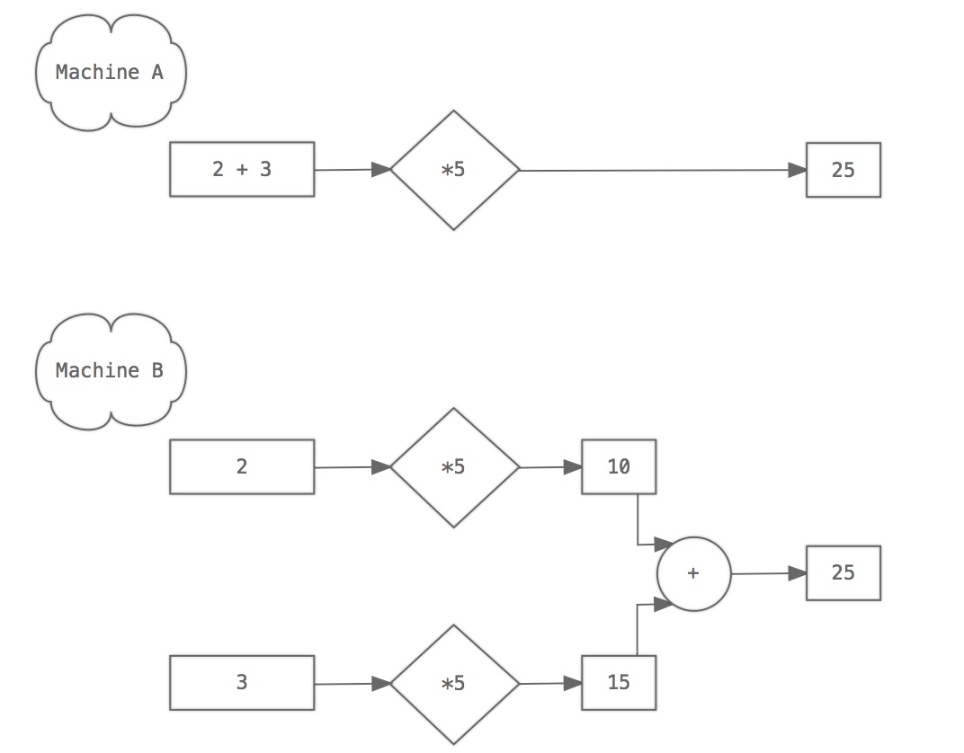
Additivity. This just means that adding two things together and then sticking them in the input will yield the same result as sticking them through individually and then adding them together afterwards. As shown below, A and B produce the same results because a times 5 number machine is additive.

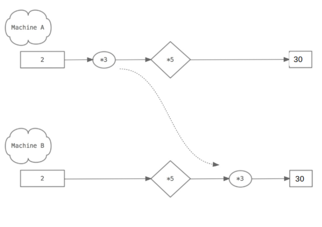
Homogeneity. This just means that a scaling coefficient applied to the input is equivalent to the same coefficient applied at the output. Again, this is shown by A producing the same result as B.

Any system that can meet these two conditions is called linear.

As for time invariance, it's exactly what it sounds like. The system doesn't change over time. Again, our number-machine above is time invariant. It doesn't care when you put your input in, it'll always give the same output for that input.

As an example of a non-LTI system, think of a compressor. It has an attack time, a decay time and it behaves differently at different gain levels. We can't easily model a compressor of any quality with convolution.

How about other tools in your standard music production kit? High Pass, Low Pass, Band Pass, (…etc) Filters, EQs, even comb filters, reverbs, delays …the list goes on. Provided none of the parameters are modulated, provided they are linear and they don't change with time, those can all be modelled with convolution! So, it looks like convolution might be pretty handy.

There is a caveat here: Modelling something like a delay with a feedback >= 100% would hypothetically require an infinitely long impulse response. (we'll get to IRs shortly) So people don't really use convolution for delays so much. We could call convolution a FIR (Finite Impulse Response) filter. Any filter that uses feedback, including most implementations of delays, HPF, LPF, combs, flangers, etc, are what we call IIR (Infinite Impulse Response) filters.

Furthermore, saying that something can be modelled with convolution is not to say it should be. There are more efficient, more sensible ways to do a lot of these things. None the less, in many cases it is possible to do so.

"What what? You just told us that a whole heap of stuff is LTI!"

So, that seems like a bit of a non-sequitur. But it's a valid question - Do LTI systems exist in reality? In the squidgy, crude, moving physical world with changing air pressure and temperature and a billion other things going on, how can there ever be a true LTI?

To cut a long story short - I don't know, but I find it hard to imagine how their could be. However, plenty of stuff is really so close to being LTI that it doesn't really matter. One example of “real things“ that are so damn close to being LTI are the reverberations of spaces. We can use convolution to capture the sound of a room. Not the sound of a specific sound in a room, but what a room would do to any sound. Kind of like stealing the room's soul. Magic, right?

Before going any further, I should point out that the mathematical operator for convolution is often drawn as an asterisk: * . This is a pain because in c++ we use that for standard multiplication (as we did above). It should be obvious from context which is intended, none the less I'll try to only use it for convolution going forward in this article.

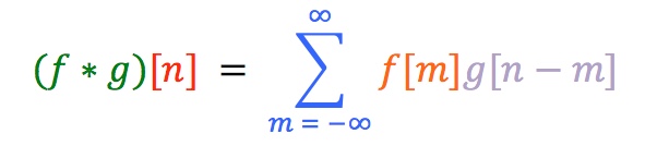
The definition of discrete-time convolution is as follows:

…and now you are thinking:

"Apart from these fun colours, this doesn't look like school-level maths at all!"

But it's really not too bad if we go step by step. What we have here is a recipe for each sample of the output of our convolution. Follow the colours:

• The nth sample of the of convolution of signals f and g is equal to (or more accurately, defined as)…
• The the sum, from m = -infinity to m = infinity, of…
• the mth sample of f times the (n-m)th sample of g

Let's translate that into more normal language:

• f[m] is really just the same as one of the input signals: f[n]. We've renamed the n axis as this new variable m doesn't change as we increment n. So our signal f stays in one place.
• g[n - m] is a back-to-front version of one of our input signals: g[n], but it moves along one step to the right every time we increment n. Why? well g[m] would be a copy of g[n], so g[-m] is a copy of g[n] but flipped around the y-axis. So, g[n-m] is that flipped version but bumped right however much we've incremented n. 

Now all together:

We keep f where it is, flip g around the y axis, bump it along n steps, and then multiply them together point-for-point:

(... g[-2]f[-2], g[-1]f[-1], g[0]f[0], g[1]f[1], g[2]f[2] ... etc )

and then add together all of those multiplications. That sum gives us the value of (f * g) at point n.

Here is the process in action:

• The blue signal is f.
• The orange signal is g (see how it gets flipped around 0 on the y axis)
• The resulting green line is the output of the convolution (f * g)

We're really imagining that our two signals are zero-padded an infinite amount at ether end. That is to say that we'd hypothetically just shove an endless line of 0s at ether end of our signal.

For example:

if g was:

[2, 3, 4]

then a infinitely zero-padded g would look like:

[...0, 0, 0, 0, 2, 3, 4, 0, 0, 0, 0, ...]

…with ether side stretching off to infinity.

In reality this is unnecessary and impractical to say the least. We'll just make sure we have enough room on ether side to capture everything.

Notice how the value of the output will always be 0 when our two input signals don't overlap (because anything times 0 is 0), and the more area under both functions on any given iteration of n, the higher the output value is at that point. Really convolution is discribing this shared area.

You can see here how the output is a bit like the two signals smudged together.

We need to flip g because we want the beginning of g to meet the beginning of f first, and the end of g to meet the end of f last, as it does in the animation above. If we didn't flip that wouldn't happen.

Also, it should be noted that it doesn't matter which signal stays still and which does the flip-and-drag. Convolution is commutative. This means that (f * g) is the same as (g * f). They make the same results. For music stuff though we're usually gonna think of one as the filter and the other as the input.

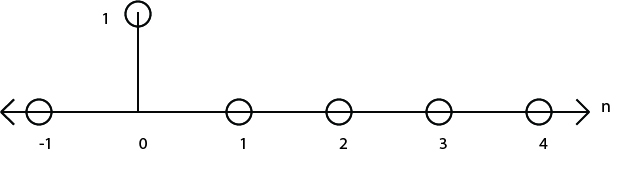
Now we know how to convolve, but how does that help us capture the reverberation of a space, or the sonic quality of a piece of hardware? To do that we need to fire off some signal in the space and record the response. We could do this with all sorts of noises and then compare the inputs to the outputs, but if we use a very specific signal as an input we can save ourselves a lot of mathematical trouble later on. Let's see how:
 An impulse (in discrete time) is a signal that is at 0 for all points apart from one point where it's value is 1. For example: [0, 1, 0, 0, 0].

The continuous time equivalent is called a Dirac delta function. Conceptually it's more complicated in continuous time and we needn't trouble ourselves with that here, but it's worth knowing the term.

This impulse is the perfect probe because it just so happens that an impulse creates every possible frequency in an equal amount. To show why that is would be a major digression here, so you'll have to take my word for it right now. When I write a post about Fourier we'll see why.

If we convolve our input signal with an impulse response if an LTI, the output is the same as though the signal had been fed into that LTI. When you think about it, any digital input signal is just a train of impulses. So it makes sense that the convolution of the signal (which is applied to every sample) creates a series of overlapping IRs that recreates the system's response to that sound.

Capturing the IR of hardware is pretty simple, we just need to input the impulse and record the response. In nature it's a bit more tricky. One of the most common methods to capture a reverb impulse response of a space is to pop a balloon and record the result. The contained, pressurised air in the ballon suddenly being exposed to the air in the space in all directions can be a decent approximation of a Dirac delta function. Of course the process of then capturing the result accurately is no doubt pretty technical and equipment intensive.